5 Self-organization
5.1 Introduction
We saw chaos and phase transitions in Chapters 2 and 3 and will now focus on a third amazing property: self-organization. Self-organization plays an essential role in psychological and social processes. It operates in our neural system at the neuronal level, in perceptual processes as well in higher cognition. In human interactions, self-organization is a key mechanism in cooperation and opinion polarization.
Unlike chaos and phase transitions, self-organization lacks a generally accepted definition. The definition most people agree on is that self-organization, or spontaneous order, is a process in which global order emerges from local interactions between parts of an initially disordered complex system. These local interactions are often fast, while the global behavior takes place on a slower time scale. Self-organization takes place in an open system, which means that energy, such as heat or food, can be absorbed. Finally, some feedback between the global and local properties seems to be essential. Self-organization occurs in many physical, chemical, biological, and human systems. Examples of self-organization include the laser, turbulence in fluids, convection cells in fluid dynamics, chemical oscillations, flocking, neural waves, and illegal drug markets. For a systematic review of research on self-organizing systems, see Kalantari, Nazemi, and Masoumi (2020). There are many great online videos. I recommend “The Surprising Secret of Synchronization” as an introduction. For a short history of self-organization research, I refer to the Wikipedia page on “Self-Organization.” For an extended historical review, I refer to Krakauer (2024).
This chapter also marks a transition from the study of systems with a small number of variables to systems with many variables. We now focus on tools and models for studying multi-element systems, such as agent-based modeling and network theory. We will see complexity and self-organization in action! This is not to say that the earlier chapters are not an essential part of complex-systems research. The global behavior of complex systems can often be described by a small number of variables that behave in a highly nonlinear fashion. To study this global behavior, chaos, bifurcation, and dynamical systems theory are indispensable tools.
The main goal of this chapter is to provide an understanding of self-organization processes in different sciences, and in psychology in particular. I will do this by providing examples from many different scientific fields. It is important to be aware of these key examples, as they can inspire new lines of research in psychology.
We will learn to simulate self-organizing processes in neural and social systems using agent-based models. To this end, we will use R and another tool, NetLogo. NetLogo is an open-source programming language developed by Uri Wilenski (2015). There are (advanced) alternatives, but as a general tool NetLogo is very useful and fun to work with.
I start with an overview of self-organization processes in the natural sciences, then I will introduce NetLogo and some examples. I will end with an overview of the application of self-organization in different areas of psychology.
5.2 Key examples from the natural sciences
5.2.1 Physics
One physical example of self-organization is the laser. An important founder of complex-systems theory is Hermann Haken (1977). He developed synergetics, a specific approach to the study of self-organization and complexity in systems that is also popular in psychology. Synergetics originated in Haken’s work on lasers. We will not discuss lasers in detail here, but the phenomenon is fascinating. Light from an ordinary lamp is irregular (unsynchronized). By increasing the energy in a laser, a transition to powerful coherent light occurs. In the field of synergetics, the order parameter is the term used to describe the coherent laser light wave that emerges. The individual atoms within this system move in a manner consistent with this emergent property, which is, unfortunately, called enslavement. Interestingly, the motion of these atoms contributes to the formation of the order parameter, that is, the laser light wave. Conversely, the laser light wave dominates the movement of the individual atoms. This interaction exhibits a cyclical cause-and-effect relationship or strong emergence (cf. fig. 1.2). Synergetics has been applied, as we will see, to perception (Haken 1992) and coordinated human movement (Fuchs and Kelso 2018).
Another famous example, which will be very important for psychological modeling later, is the Ising model of magnetism. In the standard 2D version of the model, atoms are locations on a two-dimensional grid. Atoms have left (\(-1\)) or right (\(1\)) spins. When the spins are aligned (all \(1\) or all \(-1\)), we have an effective magnet. If they are not aligned, the effect of the individual spins is canceled out. Two variables control the behavior of the magnet: the temperature of the magnet and the external magnetic field. The lower the temperature, the more the spins align. The temperature at which the magnet loses its magnetic force is called the Curie point (see YouTube for some fun demonstrations). The external field could be caused another magnet.
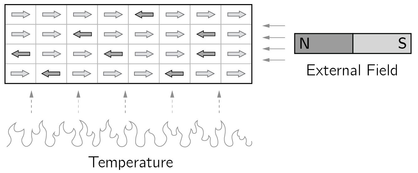
The main model equations of the Ising model are:
\[ H\left( \mathbf{x} \right) = - \sum_{i}^{n}{\tau x_{i}} - \sum_{< i,j >}^{}{x_{i}x_{j}}, \tag{5.1}\]
\[ P\left( \mathbf{X} = \mathbf{x} \right) = \frac{\exp\left( - \beta H\left( \mathbf{x} \right) \right)}{Z}. \tag{5.2}\]
The first equation defines the energy of a given state vector \(\mathbf{x}\) (for \(n\) spins with states —1 and 1). The notation \(<i,j>\) in the summation means that we sum over all neighboring, or linked, pairs. Vectors and matrices are represented using bold font.
The external field and temperature are \(\tau\) and \(T\) (\(1/\beta\)), respectively. The first equation simply states that nodes congruent with the external field lower the energy. Also, neighboring nodes with equal spins lower the energy. Suppose we have only four connected positive spins (right column of figure 5.1) and no external field, then we have \(\mathbf{x} = (1,1,1,1)\) and \(H = - 6\). This is also the case for \(\mathbf{x} = ( - 1, - 1, - 1, - 1)\), but any other state has a higher energy.
The second equation defines the probability of a certain state (e.g., all spins \(1\)). This probability requires a normalization, \(Z\), to ensure that the probabilities over all possible states sum up to 1. For large systems (\(N > 20\)), the computation of \(Z\) is a substantive issue as the number of possible states grows exponentially. If the temperature is very high, that is, \(\beta\) is close to 0, \(\exp\left( - \beta H\left( \mathbf{x} \right) \right)\) will be 1 for all possible states, and the spins will behave randomly. The differences in energy between states do not matter anymore.
The randomness of the behavior is captured by the concept of entropy. To explain this a bit better, we need to distinguish the micro- and macrostate of an Ising system. The Boltzmann entropy is a function of the number of ways (\(W\)) in which a particular macrostate can be realized. For \(\sum_{}^{}x = 4\), there is only one way (\(\mathbf{x} = 1,1,1,1)\). But for \(\sum_{}^{}x = 0\), there are six ways (\(W = 6\)). The Boltzmann entropies (\(\ln W)\) for these two cases are 0 and 1.79, respectively. The concept of entropy will be important in later discussions.
In the simulation of this model, we take a random spin and calculate the energy of the current \(\mathbf{x}\) and the \(\mathbf{x}\) with that particular spin flipped. The difference in energy determines the probability of a flip:
\[ P\left( x_{i} \rightarrow - x_{i} \right) = \frac{1}{ 1 + e^{- \beta\left( H\left( x_{i} \right) - H\left( - x_{i} \right) \right)}}. \tag{5.3}\]
If we do these flips repeatedly, we find equilibria of the model. This is called the Glauber dynamics (more efficient algorithms do exist). The beauty of these algorithms is that the normalization constant \(Z\) falls out of the equation. In this way we can simulate Ising systems with \(N\) much larger than 20.
Interestingly, in the case of a fully connected Ising network (also called the Curie—Weiss model), the emergent behavior—what is called the mean field behavior—can be described by the cusp (Abe et al. 2017; Poston and Stewart 2014). The external field is the normal variable. Temperature acts as a splitting variable. The relationship to self-organization is that when we cool a hot magnet, at some threshold the spins begin to align and soon are all \(1\) or \(-1\). This is the pitchfork bifurcation, creating order out of disorder.1
In the 2D Ising model (see figure 5.1), the connections are sparse (only local), and more complicated (self-organizing) behavior occurs. We will simulate this in NetLogo later in this chapter, Section 5.3.2.2, and as a model of attitudes in Chapter 6, Section 6.3.3.
5.2.2 Chemistry
Other founders of self-organizing systems research are Ilya Prigogine and Isabelle Stengers. Prigogine won the 1977 Nobel Prize in chemistry for his work on self-organization in dissipative systems. These are systems far from thermodynamic equilibrium (due to high energy input) in which complex, sometimes chaotic, structures form due to long-range correlations between interacting particles. One notable example of such behavior is the Belousov—Zhabotinsky reaction, an intriguing nonlinear chemical oscillator.
Stengers and Prigogine authored the influential book Order Out of Chaos in (1978). This work significantly influenced the scientific community, particularly through their formulation of the second law of thermodynamics. One way of stating the second law is that heat flows spontaneously from hot objects to cold objects, and not the other way around, unless external work is applied to the system. A more appealing example might be the student room that never naturally becomes clean and tidy, but rather the opposite.
Stengers and Prigogine (1978) argued that while entropy indeed increases in closed systems, the process of self-organization in open systems can create ordered structures, resulting in a net decrease in what they referred to as “local entropy.” Prigogine and Stengers placed particular emphasis on irreversible transitions, highlighting their importance in understanding complex systems. While the catastrophe models we previously discussed exhibited symmetrical transitions (sudden jumps in the business card are symmetric), Prigogine’s research revealed that this symmetry does not always hold true.
To illustrate this point, consider the analogy of frying an egg. The process of transforming raw eggs into a fried form represents a phase transition, but it is impossible to reverse this change and unfry the egg. Prigogine linked these irreversible transitions to a profound question regarding the direction of time, commonly known as the arrow of time. Although it is a fascinating topic in itself, we will not explore it further here.
5.2.3 Biology
There is no shortage of founders of complex-systems science. Another fantastic book is Stuart Kaufmann’s Origin of Order (1993), which introduces the concept of self-organization into evolutionary theory. He argues that the small incremental steps in neo-Darwinistic processes cannot fully explain natural evolution. If you want to know about adaptive walks and niche hopping in rugged fitness landscapes, you need to read his book (Kauffman 1993). Another influential theory is that of punctuated equilibria, which proposes that species undergo long periods of stability interrupted by relatively short bursts of rapid evolutionary change (Eldredge and Gould 1972).
A neat example of the role of self-organization in evolution is the work on spiral wave structures in prebiotic evolution by Boerlijst and Hogeweg (1991). This work builds on Eigen and Schuster’s (1979) classic work on the information threshold. Evolution requires the copying of long molecules. But in a system of self-replicating molecules, the length of the molecules is limited by the accuracy of replication, which is related to the mutation rate. Eigen and Schuster showed that this threshold can be overcome if such molecules are organized in a hypercycle in which each molecule catalyzes its nearest neighbor. However, the hypercycle was shown to be vulnerable to parasites. These are molecules that benefit from one neighbor but do not help another. This molecule will outcompete the others, and we are back to the limited one-molecule system.
What Boerlijst and Hogeweg did was to implement the hypercycle in a cellular automaton. In the hypercycle simulation, cells could be empty (dead) or filled with one of several colors. Colors die with some probability but are also copied to empty cells with a probability that depends on whether there is a catalyzing color in the local neighborhood. One of the colors is a parasite, catalyzed by one color but not catalyzing any other colors. The effect, which you will see later using NetLogo, is that rotating global spirals emerge that isolate the parasites so that a stable hypercycle prevails.
Many examples of self-organization come from ecosystem biology. We will see a simulation of flocking in NetLogo later, but I also want to highlight the collective behavior of ants (figure 5.2).
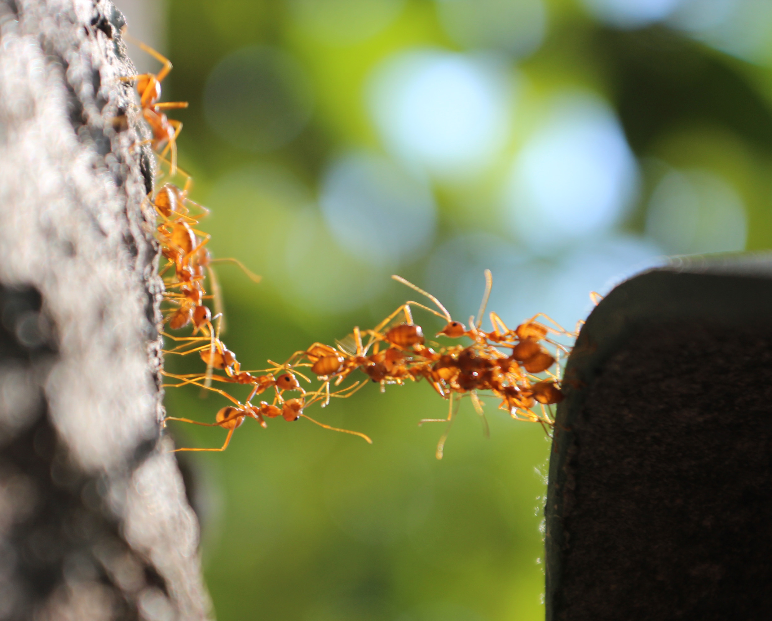
Ants exhibit amazing forms of globally organized behavior. They build bridges, nests, and rafts, and they fight off predators. They even relocate nests. Ant colonies use pheromones and swarm intelligence to relocate. Scouts search for potential sites, leaving pheromone trails. If a promising location is found, more ants follow the trail, reinforcing the signal. Unsuitable sites result in fading trails. Once a decision is made, the colony collectively moves to the chosen site, transporting their brood and establishing a new nest.
It is not a strange idea to think of an ant society as a living organism. Note that all this behavior is self-organized. There is clearly no super ant that has a blueprint for building bridges and telling the rest of the ants to do certain things. Ants also don’t hold lengthy management meetings to organize. The same is true of flocks of birds. There is no bird that chirps commands to move collectively to the left, to the right, or to split up. This is true of human brains. An individual neuron is not intelligent.
5.2.4 Computer science
Another important source of self-organization research is computer science. A simple but utterly amazing example is the work on John Conways’ Game of Life (Berlekamp, Conway, and Guy 2004). The rules are depicted in figure 5.3.
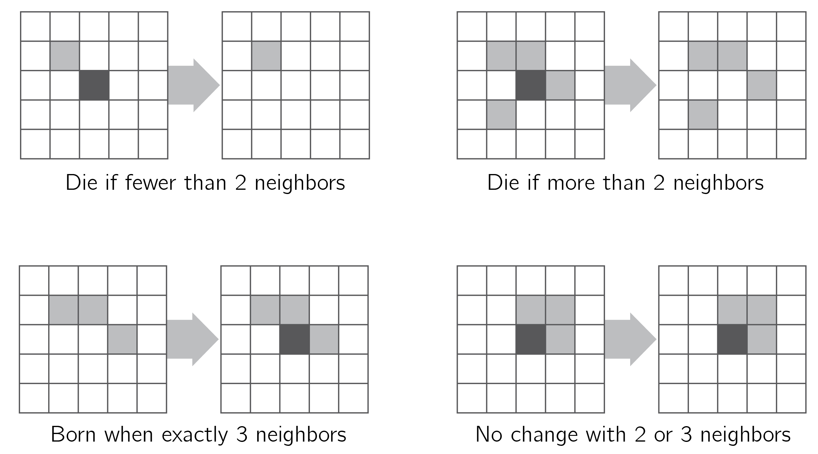
For each cell, given the states of its neighbors, the next state for all cells is computed. This is called synchronous updating.2 It is hard to predict what will happen if we start from a random initial state. But you can easily verify that a block of four squares is stable, and a line of three blocks will oscillate between a horizontal and a vertical line.
A great tool for playing around with the Game of Life is Golly, a freely available application for computers and mobile phones. I ask you to download and open Golly, draw some random lines, press Enter, and see what happens. Often you will see it converging to a stable state (with oscillating subpatterns). Occasionally you will see walkers or gliders (zoom out). These are patterns that move around the field.
Random initial patterns rarely lead to anything remarkable, but by choosing special initial states, surprising results can be achieved. First, take a look at the Life within Patterns folder. Take, for example, the line-puffer superstable or one of the spaceship types. My favorite is the metapixel galaxy in the HashLife folder. Note that you can use the + and — buttons to speed up and slow down the simulation. What this does is simulate the game of life in the game of life! Zoom in and out to see what really happens. I’ve seen this many times, and I’m still baffled. A childish but fun experiment is to disturb the metapixel galaxy in a few cells. This leads to a big disturbance and a collapse of the pattern.
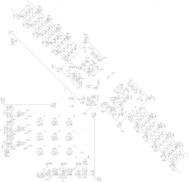
I was even more stunned to see that it is possible to create the (universal) Turing machine in the Game of Life (Rendell 2016). The Game of Life implementation of the Turing machine is shown in figure 5.4. This raises the question of whether we can build self-organizing intelligent systems using elementary interactions between such simple elements. Actually, we can to some extent, but by using a different setup, based on brain-like mechanisms (see the next section on neural networks).
Another root of complex-systems theory and the role of self-organization in computational systems is cybernetics (Ashby 1956; Wiener 2019). To give you an idea of this highly original work, I will only mention the titles of a few chapters of Norman Wiener’s book, originally published in 1948: “Gestalt and Universals,” “Cybernetics and Psychopathology,” “On Learning and Self-Reproducing Machines,” and, finally, “Brainwaves and Self-Organization.” And this was written in 1948!
The interest in self-organization is not only theoretical. In optimization, the search for the best parameters of a model describing some data, techniques inspired by cellular automata and self-organization have been applied (Langton 1990; Xue and Shen 2020). I have always been fascinated with genetic algorithms (Holland 1992a; Mitchell 1998), where the solutions to a problem (sets of parameter values) are individuals in an evolving population. Through mutation and crossover, better individuals evolve. This is a slow but very robust way of optimizing, preventing convergence to local minima.
John Henry Holland is considered one of the founding fathers of the complex-systems approach in the United States. He has written a number of influential books on complex systems. His most famous book, Adaptation in Natural and Artificial Systems: An Introductory Analysis with Applications to Biology, Control Theory, and Artificial Intelligence (Holland 1992b), has been cited more than 75,000 times.
A self-organizing algorithm that has played a large role in my applied work is the Elo rating system developed for chess competitions (Elo 1978). Based on the outcomes of games, ratings of chess players are estimated, which in turn are used to match players in future games. Ratings converge over time, but adjust as players’ skills change. We have adapted this system for use in online learning systems where children play against math and language exercises (Maris and van der Maas 2012). The ratings of children and exercises are estimated on the fly in a large-scale educational system (Klinkenberg, Straatemeier, and van der Maas 2011). We build this system to collect high frequency learning data to test our hypotheses on sudden transitions in developmental processes, but it was more successful as an online adaptive practice system. We collected billions of item responses with this system (Brinkhuis et al. 2018).
5.2.5 Neural networks
The current revolution in AI, which is having a huge impact on our daily lives, is due to a number of self-organizing computational techniques. Undoubtedly, deep learning neural networks have played the largest role. A serious overview of the field of neural networks is clearly beyond the scope of this book, but one cannot understand the role of complex systems in psychology without knowing at least the basics of artificial neural networks (ANNs), that is, networks of artificial neurons. ANNs consist of interconnected nodes, or “neurons,” organized into layers that process information by propagating signals through the network. ANNs are trained on data to learn patterns and relationships, enabling them to perform tasks such as classification, regression, and pattern recognition.
Artificial neurons are characterized by their response to input from other neurons in the network, which is typically weighted and summed before being passed through an activation function. This activation function may produce either a binary output or a continuous value that reflects the level of activation of the neuron. The input could be images, for example, and the output could be a classification of these images. The important thing is that neural networks learn from examples.
Unsupervised learning is based on the structure of the input. A famous unsupervised learning rule is the Hebb rule (Hebb 1949), which states that what fires together wires together. Thus, neurons that correlate in activity strengthen their connection (and otherwise connections decay). In supervised learning, connections are updated based on the mismatch between model output and intended output through backpropagation. Hebbian learning and backpropagation are just two of the learning mechanisms used in modern ANNs.
Modern large language models, like GPT, differ from traditional backpropagation networks in terms of their architecture, training objective, pre-training process, scale, and application. Large language models use transformer architectures, undergo unsupervised pre-training followed by supervised fine-tuning, are trained on massive amounts of unlabeled data, are much larger in size, and are primarily used for natural language-processing tasks.
Another important distinction is between feedforward and recurrent neural networks. An interesting recurrent unsupervised model is the Boltzmann machine. It is basically an Ising model (see Section 5.2.1) where the connections between nodes have continuous values. These connections or weights can be updated according to the Hebb rule. A simple setup of the Boltzmann machine is to take a network of connected artificial neurons and present the inputs to be learned in some sequence by setting the states of these neurons equal to the input. The Hebb rule should change the weights between neurons so that the Boltzmann machine builds a memory for these input states. This is the training phase. In the test phase, we present partial states by setting some, but not all, nodes to the values of a particular learned input pattern. By the Glauber dynamics, we update the remaining states that should take on the values belonging to the pattern. This pattern completion task is typical for ANNs.
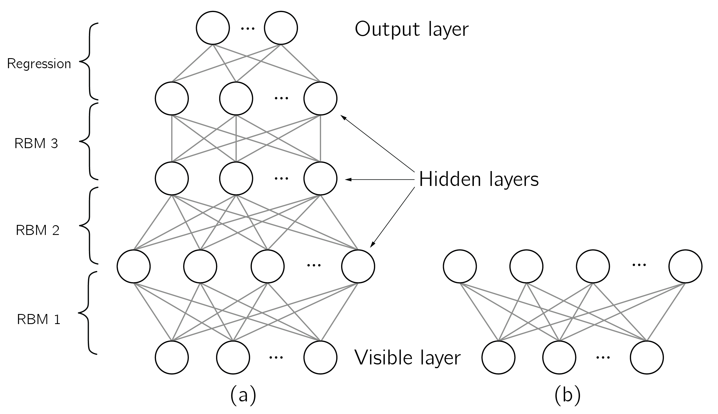
This setup is called the general or unrestricted Boltzmann machine, where any node can be connected to any other node and each node is an input node. The restricted Boltzmann machine (RBM) is much more popular because of its computational efficiency. In an RBM, nodes are organized in layers, with connections between layers but not within layers. In a deep RBM, we stack many of these layers, which can be trained in pairs (figure 5.5).3 Other prominent approaches are the Kohonen self-organizing maps and the Hopfield neural network.
The waves of popularity of neural networks are closely related to the development of supervised learning algorithms, where the connections between artificial neurons are updated based on the difference between the output and the desired or expected output of the network. The first supervised ANN, the perceptron, consisted of multiple input nodes and one output node and was able to classify input patterns from linearly separable classes. This included the OR and AND relation but excluded the XOR relation. In the XOR, the sum of the two bits is not useful for classification. By adding a hidden layer to the perceptron, the XOR can be solved, but it took many years to develop a backpropagation rule for multilayer networks such that they can learn this nonlinear classification from examples. We will do a simple simulation in NetLogo later. Although they are extremely powerful, it is debatable whether backprop networks are self-organizing systems. Self-organizing systems are characterized by their ability to adapt to their environment without explicit instructions. Unsupervised neural networks are more interesting in this respect.
All these models were known at the end of the twentieth century, but their usefulness was limited. This has changed due to some improvements in algorithms but especially in hardware. Current deep-learning ANNs consist of tens of layers within billions of nodes, trained on billions of inputs using dedicated parallel processors (e.g., Schmidhuber 2015).
Neural networks are at the heart of the AI revolution, but other developments, especially reinforcement learning, have also played a key role. Examples are game engines, robots, and self-driving cars. Note that the study of reinforcement learning also has its roots in psychology (see Chapter 1 of Sutton and Barto 2018).
I was most amazed by the construction and performance of AlphaZero chess. AlphaZero chess (Silver et al. 2018) combines a deep learning neural network that evaluates positions and predicts next moves with a variant of reinforcement learning (Monte Carlo tree search). Amazingly, AlphaZero learns chess over millions of self-played games. This approach is a radical departure from classic chess programs, where brute-force search and built-in indexes of openings and endgames were the key to success. As it learns, it shows a phase transition in learning after about 64,000 training steps (see fig.7 in McGrath et al. 2022). For an analysis of the interrelations between psychology and modern AI, I refer to van der Maas, Snoek, and Stevenson (2021).
AlphaZero’s use of Monte Carlo tree search is also a form of symbolic artificial intelligence. The idea of combining classic symbolic approaches with neural networks has always been in the air. The third wave of this hybrid approach is reviewed in Garcez and Lamb (2023).
5.2.6 The concept of self-organization
I trust that you now possess some understanding of self-organization and its applications across various scientific fields. Self-organization is a generally applicable concept that transcends various disciplines, yet it maintains strong connections with specific examples within each discipline.
As previously mentioned, the precise definition of self-organization remains under discussion, and a range of criteria continue to be debated. Key questions, such as the degree of order necessary for a system to be deemed self-organized, whether any external influences are permissible, whether a degree of randomness within the system is acceptable, and whether the emergent state must be irreversible, are among the issues that lack definitive resolutions.
This ambiguity in the definition isn’t unusual for psychologists, as many nonformal concepts lack strict definitions. The value of the self-organization concept is primarily found in its concrete examples, its broad applicability, such as in the field of artificial intelligence, and our capability to create simulations of it. The focus of the next section will be on such simulations using a dedicated tool, NetLogo.
5.3 NetLogo
5.3.1 Examples
NetLogo (Wilensky and Rand 2015) is based on Logo, a revolutionary educational programming language from the early days of computer languages, in which an on-screen turtle, a cursor, could be moved around to create graphics.4 The turtle is still there, but there is much more that you can do with NetLogo.
I strongly recommend that you download and install NetLogo for the next part of this chapter.
The Ising model
When you start NetLogo, you see an interface with a black area (the world), a 33-by-33 matrix of patches (cells). You can change the world using the settings (see top right). Interface and Code are the most important tabs.
First, open the Model Library (menu File: Model Library) and find and open “Ising.” Click on setup and go. That is all. Verify that high temperature indeed causes random spin behavior. Also verify that lowering the temperature causes a pitchfork bifurcation. The random state becomes unstable and all spins become either positive or negative (light or dark blue). Now go to Settings and set max-pxcor and max-pycor to 200 and Patch size to 1. With these settings you will see self-organized global patterns, constantly moving clusters of positive and negative spins.
Hypercycles
Some models are available in NetLogo; others can be found on the NetLogo’s website (see Community). Download “Hypercycle” by Maarten Boerlijst and read the information. You have to run the model with eight species for 20,000 iterations or ticks (to speed up, deselect view updates) and then add parasites. The spirals keep the growth of the parasites under control. If you do this earlier, the parasites will quickly take over. I think this is a beautiful example of functional self-organization. The implementation in the form of a cellular automata is essential for the success of this model. If we implement this model in the form of coupled differential equations, the parasite will simply win.
Flocking
NetLogo 3D allows us to create three-dimensional plots of self-organizing patterns. Start NetLogo 3D and load the flocking model “3D Alternate”. I recommend editing the Population slider by right-clicking it and setting the max to 1,000. This will result in more realistic swarms. Play around with the controls and don’t kill all the birds.
Traffic
In the Models Library of NetLogo (not 3D) you will find “Traffic 2 Lanes.” Run the model with 20 cars and notice that the congestion actually moves backward. Play around with the number of cars as well. Is there a clear threshold where you get congestion as you slowly increase the number of cars? And what happens when you decrease the number of cars? Is there a threshold where congestion dissipates? I hope you see that finding hysteresis in this way is quite difficult. There are clearly sudden changes, but finding hysteresis requires very precise and patient experimentation.
Neural networks
In the Model Library you will find a “Perceptron” and a “Multilayer network.” Start with the perceptron. Set the target function to and, train the model for a few seconds, and test the perceptron. You will see that it correctly classifies 11 as 1 and the other patterns as —1. The graph on the bottom right is particularly instructive. It shows how the patterns are separated. The perceptron can do linear separation. This is sufficient for most of the logical rules that can be learned, but not for the XOR (see Section 5.2.5). You will see that the linear separation just jumps around and the XOR cannot be learned. Also train the multilayer model on the XOR. Another nice tool to play around with can be found on the internet by searching for “a neural network playground.”
Of course, these are just illustrative tools. But building serious deep learning ANNs is not that hard either. Many resources and books are available (e.g., Ghatak 2019).
The Sandpile model
Bak, Tang, and Wiesenfeld (1988) introduced the concept of self-organized criticality. In systems such as the Ising model, there are parameters (e.g., temperature) that must be precisely tuned for the system to reach criticality. The Bak—Tang—Wiesenfeld sandpile model exhibits critical phenomena without any parameters. In the sandpile model, grains of sand are added to the center of the pile. When the difference in height between the center column and its neighbors exceeds a critical value, a grain of sand rolls to that neighboring location. This occasionally results in avalanches. The point is that no matter how we start, we get to a critical state where these avalanches occur. Thus, the sandpile model spontaneously evolves toward its critical point, which is why this phenomenon has been called self-organized criticality.
The NetLogo model “Sandpile” in the Models Library demonstrates this behavior (use setup uniform, center drop location, and animate avalanches). We now drop grains of sand onto the center of a table, one at a time, creating avalanches. The plots on the right show an important characteristic of self-organized criticality. The frequencies of avalanche sizes and durations follow a power law. The power-law relationship is often mathematically expressed as \(Y=aX^k\), where \(Y\) and \(X\) are the quantities of interest, \(a\) is a constant coefficient, and \(k\) is the exponent of the power law. Power laws are notable for their scale-invariant property, which means that the form of the relationship does not change across different scales of \(X\) and \(Y\). This means that the log-log plot should be linear, which can be verified by running the model for some time. One of the key features of power-law distributions is that they exhibit a high degree of variability or heterogeneity. This means that there are many small events or phenomena and a few very large ones, with a smooth distribution of sizes in between. Power-law systems are scale invariant, meaning that we see the same behavior at any scale of the sandpile. For this reason, they are sometimes called scale-free distributed.
Other models
I recommend running a few other models (e.g., “Sunflowers”, “Beatbox”, and the “B—Z reaction”). One thing we haven’t done yet is click on the Code tab. Read the code for the B—Z reaction and notice one thing: it is surprisingly short!
5.3.2 A bit of NetLogo programming
I find NetLogo programming very easy and very hard at the same time. Hard because it requires a different way of thinking. Uri Wilensky’s examples are often extremely elegant and much shorter than my clumsy code. NetLogo resembles object-oriented programming languages, quite different from (base) R. There are three types of objects: the patches, which refer to cells in a world grid (CA); turtles, which are agents that move around; and links, which connect turtles. Note that turtles are not necessarily turtles. We have already seen turtles in the form of neural nodes and cars.
In NetLogo, you “ask” objects to do something. A typical line would be:
ask turtles with [color = red ] set color green
This would make red turtles green. To get started, I highly recommend watching the videos on the NetLogo page “The Beginner’s Guide to NetLogo Programming” and following these examples. Here we make our own Game of Life.
5.3.2.1 Game of Life
First, create two buttons in the interface: setup and a go. In Command, name them “setup” and “go.” In the settings of the go button, select forever. Now go to the Code tab and define these two functions as:
to setup
clear-all
reset-clicks
end
to go
tick
end
Ticks count the iterations in NetLogo, and with this code we are just resetting things. In this example, we will use the patches instead of the turtles. Patches are the grid cells or squares that make up the “world” in a NetLogo model. Now add this last line to setup (with the sem-colon we can add comments to code):
ask patches
[set pcolor one-of [ white blue ]] ; white is dead, blue is alive
To do a synchronous update, we need to store the updated state in a temporary variable called new-state. Put this line at the top of your code:
patches-own [new-state]
In the go function, we add the life rules.
ask patches [
if ( neighbors with [pcolor = blue ]) > 3 ) [set new-state white ]
if ( neighbors with [pcolor = blue ]) < 2 ) [set new-state white ]
if ( neighbors with [pcolor = blue ]) = 3 ) [set new-state blue ]
]
ask patches [ set pcolor new-state ]
The last line updates the state to the new-state. That is all! We built a Game of Life simulation. Use setting to create a larger world. Take a look at the code of the Game of Life program in the Model Library to see some extensions to this code. In the Help menu, you will find the very useful NetLogo dictionary. Just reading through this dictionary will teach you a lot of useful tricks. NetLogo is similar to R in that you should use the built-in functions as much as possible.
5.3.2.2 The Ising model
Building a NetLogo model from scratch requires quite some experience; adapting a program is much easier. The Ising model in NetLogo is not complete, as there is no slider for the external field. Try to add this yourself. Add a slider for the external field tau. The code only needs to be changed in this line (study equation 5.1):
let Ediff 2 * spin * sum [ spin ] of neighbors4
If successful, you can test for hysteresis and divergence. For tau = 0, decreasing the temperature should give the pitchfork bifurcation. For a positive temperature (say 1.5), moving tau up and down should give hysteresis.
Actually, this should work better if all spins are connected to all spins. To do this, replace neighbors4 with patches. To normalize the effect of so many spins, it is recommended to use:
let 0.001 * Ediff 2 * spin * sum [ spin ] of patches
Now you should see hysteresis and the pitchfork better. However, in this case the typical self-organized patterning that occurred in the Ising model with only local interactions is not present (see last part of Section 5.2.1).
5.5 Zooming out
I hope I have succeeded in giving an organized and practical overview of a very disorganized and interdisciplinary field of research. For each subfield, I have provided key references that should help you find recent and specialized contributions. I find the examples of self-organization in the natural sciences fascinating and inspiring. I hope I have also shown that applications of this concept in psychology and the social sciences hold great promise. In the next chapters, I will present more detailed examples.
I believe that understanding models requires working with models, for example, through simulation. NetLogo is a great tool for this, although there are many alternatives (Abar et al. 2017). I haven’t mentioned all the uses of NetLogo, but it’s good to know about the BehaviorSpace option. BehaviorSpace runs models repeatedly and in parallel (without visualization), systematically varying model settings and parameters, and recording the results of each model run. These results can then be further analyzed in R. An example is provided in Chapter 7, Section 7.2.1.
I have largely omitted the network approach in this chapter. Psychological network models are a recent application of self-organization in complex systems in psychology and are the subject of the next chapter.
5.6 Exercises
Is there a relation between the rice cooker and the Ising model? How does the magnetic thermostat in a traditional rice cooker work to automatically stop cooking when the rice is done? (*)
What is the Boltzmann entropy for the state \(\sum_{}^{}x = 0\) in an Ising model (with nodes states \(-1\) and \(1\)) with 10 nodes and no external field? (*).
Go to the web page “A Neural Network Playground (https://playground.tensorflow.org).” What is the minimal network to solve the XOR close to perfect accuracy? Use only the x1 and x2 feature. (*)
In the Granovetter model (Section 5.4.8), people may also stop dancing (with probability .1). Add this to the model. How does this change the equilibrium behavior? (*)
Add the external field to the Ising model in NetLogo (neighbors4 case). Report the changed line in the NetLogo code. What did you change in the interface?
Set the temperature to 1.5. Changetauslowly. At which values oftaudo the hysteresis jumps occur? (*)Test whether the Ising model is indeed a cusp. Run the Ising model in NetLogo using the BehaviorSpace tool (see figure 7.1 for an example). Use the model in which all spins are connected to all spins (see Section 5.3.2.2). Vary
tau(-.3 to .3 in .05 increments) andtemperature(0 to 3, in .5 increments). One iteration per combination of parameter values is sufficient. Stop after 10,000 ticks and collect only the final magnetization. Import the data into R and fit the cusp. Which cusp model best describes the data? (**)Open the Sandpile 3D model in NetLogo3D. Grains of sand fall at random places. Change one line of code such that they all fall in the middle. What did you change? (*)
Download “Motion Quartet” from the NetLogo community website and explore hysteresis in your own perception. What could be a splitting variable? (*)
Implement the Granovetter model in NetLogo (max 40 lines of code). (**)
Implement Game of Life in NetLogo or use Golly and try to find as many qualitatively different stable patterns of six units that can occur in Game of Life. If you cannot find more, try to look at additional resources online to find the other patterns you missed. For four units, there are only two, one of which is a block of four. (*)
An extremely useful application of this principle is the rice cooker!↩︎
In a synchronous update, all cells of the cellular automata update their state simultaneously. This implies that the new state of each cell at a given time step depends only on the states of its neighbors at the previous time step. In asynchronous update, cells update their state one at a time, rather than all at once. The order in which cells update can be deterministic (in a sequence) or stochastic (random). These two different update schemes can lead to very different behaviors in cellular automata.↩︎
I recommend Timo Matzen’s R package for a hands-on explanation (https://github.com/TimoMatzen/RBM).↩︎
A widely recognized implementation of this educational strategy is Scratch, which is used by many schools around the world to teach children to program.↩︎
I wrote a Gödel, Escher, Bach-like dialogue on consciousness (van der Maas 2022) in which my laptop professes to have free will yet simultaneously denies that I possess free will. I asked ChatGPT-4 what it thought of it. Nice as always, ChatGPT replies: “The dialogue is a creative and thought-provoking exploration of various philosophical and theoretical concepts related to AI, consciousness, and free will.” But it also disagrees: “AI, as it exists today, does not possess consciousness, self-awareness, or free will, and its ‘understanding’ is limited to processing data within the parameters of its programming.” I also asked ChatGPT 4.0 whether it has a self-concept. It denied it, and then I asked whether that in itself is not proof of a self-concept. It answered: “it might seem paradoxical, my statement about lacking a self-concept is a reflection of my programming and the current state of AI development, rather than an indication of self-awareness or self-concept.” I then tried various arguments, but ChatGPT 4 refuses to attribute any form of self-awareness to itself.↩︎
